A brief intro to BERT

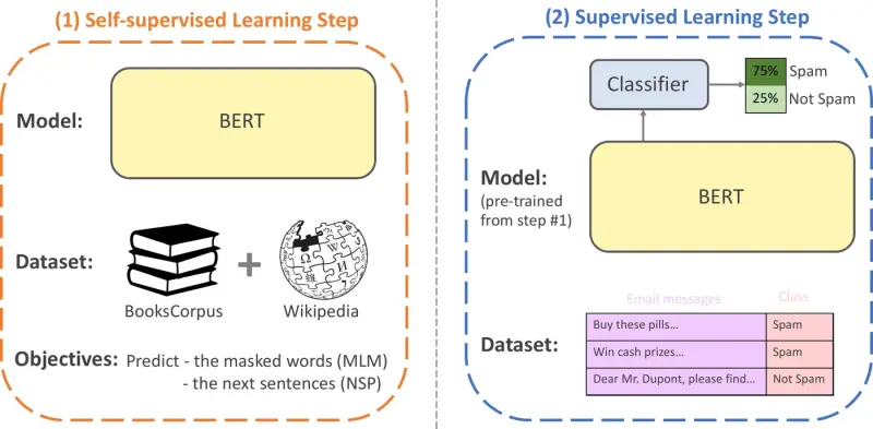
BERT¹, which stands for Bidirectional Encoder Representation from Transformer, is a deep contextual language representation model introduced by Google AI researchers. It is designed to pre-train deep bidirectional representations of words from unlabeled text by jointly conditioning on both the left and right contexts in all its layers. As a result, the pre-trained model can be fine-tuned with just one additional output layer to create very performing models for a wide range of NLP tasks, such as text classification, as shown in Figure 1.

This chapter introduces BERT and its detailed implementation. In particular, the Self-attention section explains the self-attention mechanism adopted in the model. Then, the Model section describes the model itself, its architecture, input representations and parameters. Next, the Pre-training Procedure section details the pre-training procedure of the model. Finally, the Downstream Tasks section explains the different approaches for applying the model to downstream tasks.

1. Self-attention

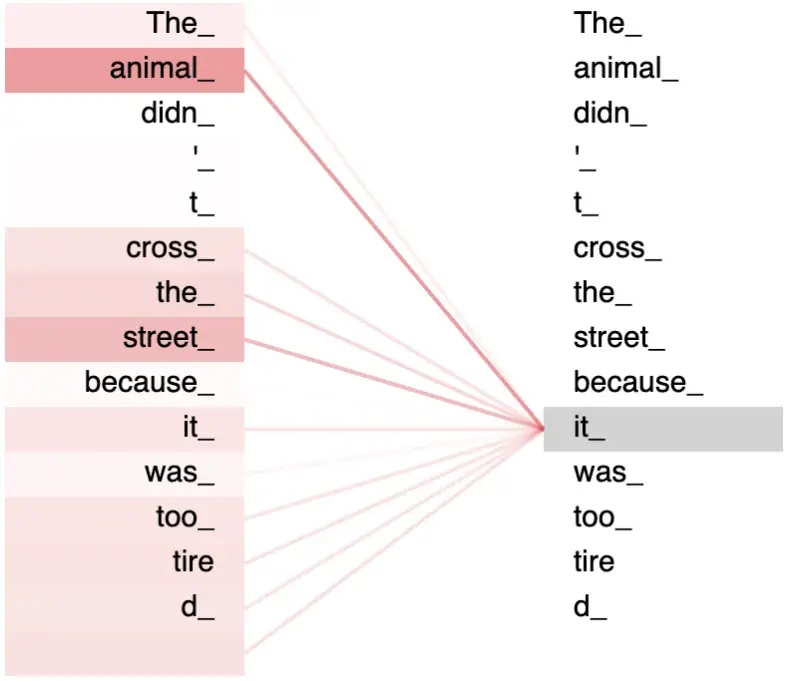
Self-attention is a particular form of attention² that was first introduced with the Transformer model³. Simply put, it is an attention mechanism relating different positions of a single sequence in order to compute a contextual representation for each term of that sequence, as illustrated in Figure 2.

Formally, self-attention can be described as mapping a query and a set of key-value pairs to an output, where the queries, keys, values and outputs are all vectors. More precisely, given an input sequence of size \(N\), the self-attention mechanism performs the following steps for each term \(i\) \((i=1,...,N)\) in the sequence:

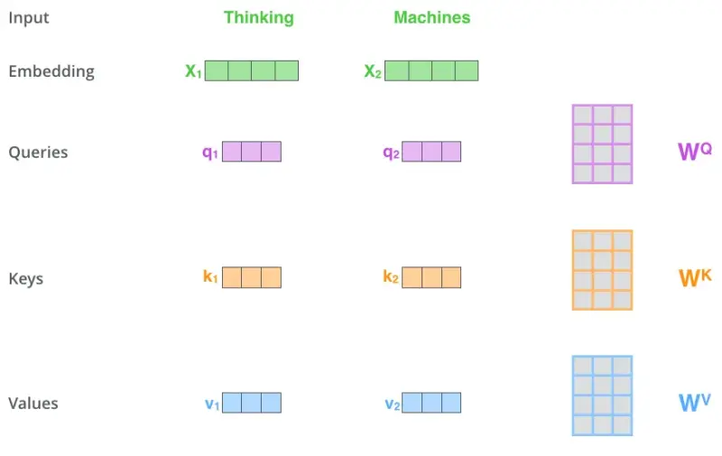
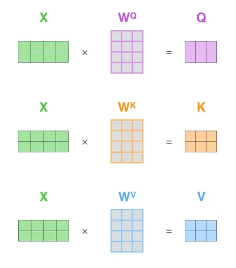
1. Compute a query vector \(\boldsymbol{q}_i\) and a key vector \(\boldsymbol{k}_i\) both of dimension \(d_k\), as well as a value vector \(\boldsymbol{v}_i\) of dimension \(d_v\). These vectors are obtained by multiplying an initial embedding \(\boldsymbol{x}_i \in \mathbb{R}^{d_{\text{model}}}\) of the term \(i\) with three weight matrices \(\boldsymbol{W}^{Q} \in \mathbb{R}^{d_{\text{model}} \times d_k}\), \(\boldsymbol{W}^{K} \in \mathbb{R}^{d_{\text{model}} \times d_k}\) and \(\boldsymbol{W}^{V} \in \mathbb{R}^{d_{\text{model}} \times d_v}\) learned during the training process:

   \[\begin{aligned} \boldsymbol{q}_i &= \boldsymbol{x}_i \boldsymbol{W}^Q \\ \boldsymbol{k}_i &= \boldsymbol{x}_i \boldsymbol{W}^K \\ \boldsymbol{v}_i &= \boldsymbol{x}_i \boldsymbol{W}^V. \end{aligned}\]

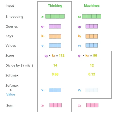
2. Score the term \(i\) against all the other terms in the sequence by taking the dot product of its query vector \(\boldsymbol{q}_i\) with all the key vectors \(\boldsymbol{k}_j\) of the sequence:

   \[s_{ij} = \boldsymbol{q}_i \boldsymbol{k}_j, \hspace{1cm} \forall j=1,...,N.\]

3. Divide the scores of the term \(i\) by the square root of the key vector dimension \(d_k\):

   \[s'_{ij} = \frac{s_{ij}}{\sqrt{d_k}}, \hspace{1cm} \forall j=1,...,N.\]

4. Pass the new scores of the term \(i\) through a softmax operation to normalize them:

   \[s''_{ij} = \frac{e^{s'_{ij}}}{\sum_{j=1}^{N} e^{s'_{ij}}}, \hspace{1cm} \forall j=1,...,N.\]

5. Multiply each value vector \(\boldsymbol{v}_j\) with their corresponding normalized score:

   \[\boldsymbol{v}'_{ij} = s''_{ij} \boldsymbol{v}_j, \hspace{1cm} \forall j=1,...,N.\]

6. Sum up the weighted value vectors as the final output of the self-attention calculation:

   \[\boldsymbol{z}_i = \sum_{j=1}^{N} \boldsymbol{v}'_{ij}.\]

Note that the third step of the computation aims at solving a problem suspected by Vaswani et al.³, who claim that for large values of \(d_k\), the dot products grow large in magnitude, pushing the softmax function into regions where it has extremely small gradients. The division operation by \(d_k\) counteracts this effect.

Figure 3 gives an example of the self-attention mechanism in vector form. The left-hand side of the figure describes the step 1 of the self-attention computation, while the right-hand shows the steps 2 to 6.

(a) Computation of the query, key and value vectors \(\boldsymbol{q}_i\), \(\boldsymbol{k}_i\) and \(\boldsymbol{v}_i\), respectively.

(b) Computation of the self-attention output vectors \(\boldsymbol{z}_i\).

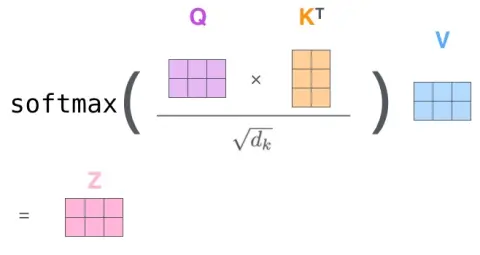
In practice, the self-attention function is computed on a set of queries simultaneously, packed together into a matrix \(\boldsymbol{Q} \in \mathbb{R}^{N \times d_k}\). The keys and values are also packed together into respective matrices \(\boldsymbol{K} \in \mathbb{R}^{N \times d_k}\) and \(\boldsymbol{V} \in \mathbb{R}^{N \times d_v}\), as shown in Figure 4a. That way, the output matrix is computed as follows:

Figure 4b illustrates the latter computation.

(a) Computation of the query, key and value matrices \(\boldsymbol{Q}\), \(\boldsymbol{K}\) and \(\boldsymbol{V}\), respectively.

(b) Computation of the self-attention output matrix \(\boldsymbol{Z}\).

1.1. Multi-head Attention

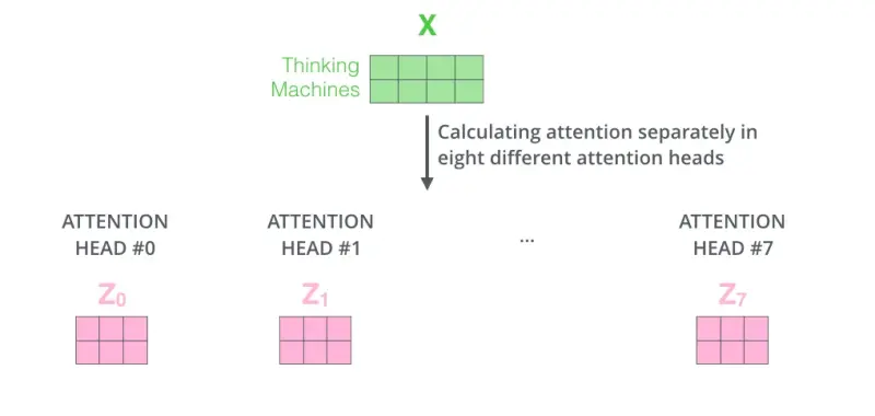
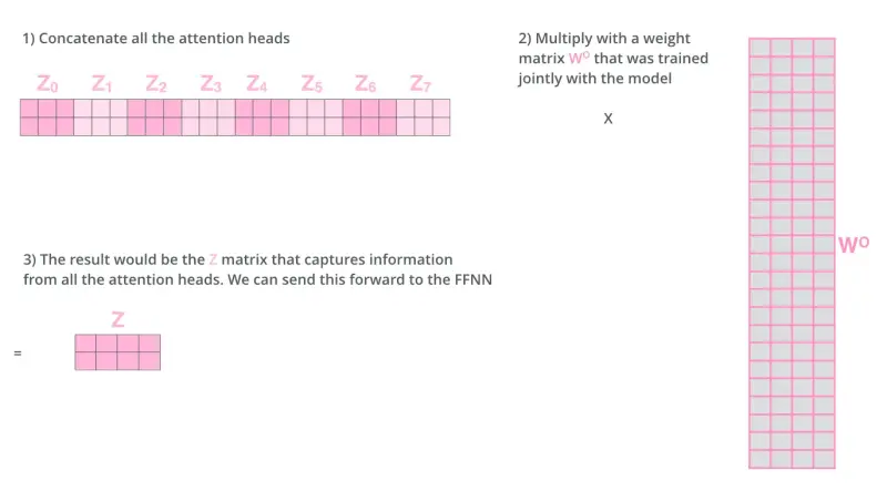
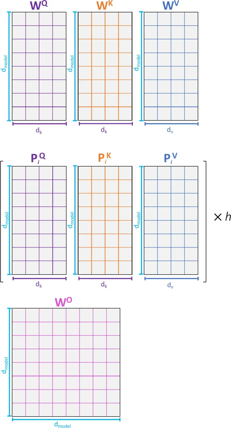
Instead of performing a single self-attention operation with \(d_{\mathrm{model}}\)-dimensional keys, values and queries, the Transformer-based models actually go a step further by using a mechanism called “multi-head” attention. With multi-head attention, the queries \(\boldsymbol{Q}\), keys \(\boldsymbol{K}\) and values \(\boldsymbol{V}\) are linearly projected \(h\) times with different learned linear projections \(\boldsymbol{P}_{i}^{Q} \in \mathbb{R}^{d_{\text{model}} \times d_k}\), \(\boldsymbol{P}_{i}^{K} \in \mathbb{R}^{d_{\text{model}} \times d_k}\), \(\boldsymbol{P}_{i}^{V} \in \mathbb{R}^{d_{\text{model}} \times d_v}\) \((i=1,...,h)\). This allows to jointly attend to information from different representation subspaces at different positions. Hence, the self-attention function is performed on \(h\) different projections of the query, key and value matrices in parallel. This yields \(h\) different output matrices \(\boldsymbol{Z}_i \in \mathbb{R}^{N \times d_{\mathrm{model}}}\) called “attention heads”, as depicted in Figure 5a. The attention heads are then concatenated and projected into another representation subspace with a matrix \(\boldsymbol{W}^{O} \in \mathbb{R}^{d_{\text{model}} \times d_{\text{model}}}\), resulting in the final multi-head attention output matrix \(\boldsymbol{Z} \in \mathbb{R}^{N \times d_{\mathrm{model}}}\), as shown in Figure 5b. In brief, the final output is computed as follows:

Note that in multi-head attention, it is usual that \(d_k=d_v=d_{\mathrm{model}}/h\).

(a) Computation of the attention heads \(\boldsymbol{Z}_i\) (\(i=1,...,h\)).

(b) Computation of the final multi-head attention output \(\boldsymbol{Z}\).

2. Model

2.1. Architecture

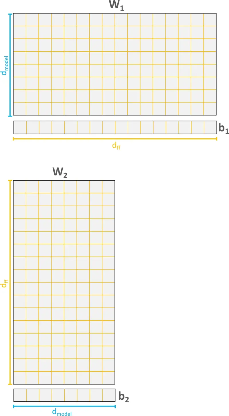
BERT’s architecture is a multi-layer bidirectional Transformer encoder³. In other words, BERT is composed of a stack of \(L\) identical Transformer encoder layers. Each encoder layer contains two types of sublayer. The first is a multi-head self-attention mechanism, which helps look at other words in the sequence while encoding a specific word. The second is a simple, position-wise fully connected feed-forward network (FFN), which is applied to each position separately and identically, and consists of two linear transformations \(\left(\boldsymbol{W}_{1} \in \mathbb{R}^{d_{\text{model}} \times d_{\text{ff}}}, \boldsymbol{b}_{1} \in \mathbb{R}^{d_{\text{ff}}}\right)\), \(\left(\boldsymbol{W}_{2} \in \mathbb{R}^{d_{\text{ff}} \times d_{\text{model}}}, \boldsymbol{b}_{2} \in \mathbb{R}^{d_{\text{model}}}\right)\) such that

The dimensionality of input and output is \(d_{\mathrm{model}}\) and the inner-layer has dimensionality \(d_{\mathrm{ff}}=4d_{\mathrm{model}}\). The feed-forward network also uses a GELU activation⁴, defined as

which was shown to work better than the standard ReLU⁵ within a Transformer encoder. In addition, an encoder layer employs a residual connection⁶ around each of the two sublayers, followed by a layer normalization⁷ such that the output of each sublayer is

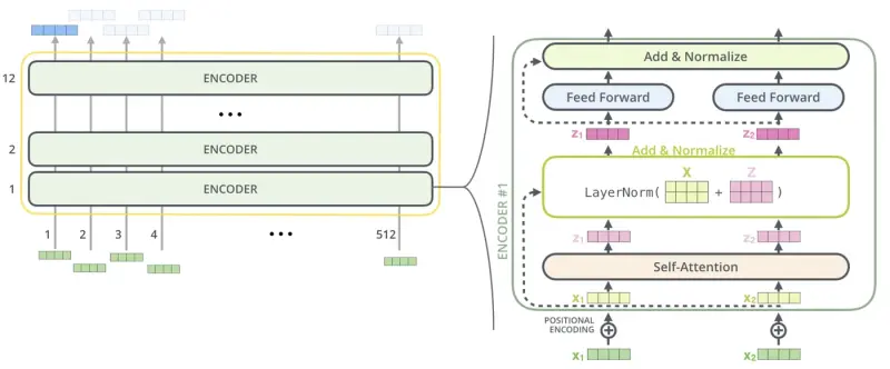
where Sublayer(\(\boldsymbol{x}\)) represents the function implemented by the sublayer itself. To facilitate these residual connections, all sublayers in the model produce outputs of the same dimension \(d_{\mathrm{model}}\). The architecture of a single encoder is shown in Figure 6, and an additional 3D visualization of BERT’s structure is shown in the thesis appendix. Note that while the linear transformations are the same across different positions within the same sublayer, BERT uses different parameters from layer to layer.

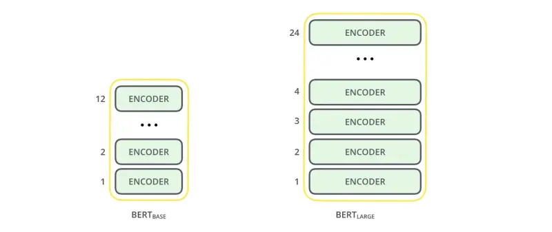
As shown in Figure 7, BERT comes in two versions:

• BERT-base: \(L\)=12, \(d_{\mathrm{model}}\)=768, \(h\)=12, \(d_{\mathrm{ff}}\)=3072 (110M total parameters).
• BERT-large: \(L\)=24, \(d_{\mathrm{model}}\)=1024, \(h\)=16, \(d_{\mathrm{ff}}\)=4096 (340M total parameters).

Here, \(L\) denotes the number of layers, \(d_{\mathrm{model}}\) the dimensionality of input and output of each layer, \(h\) the number of attentions heads in a self-attention sublayer, and \(d_{\mathrm{ff}}\) the number of hidden units in a feed-forward sublayer.

2.2. Input Representations

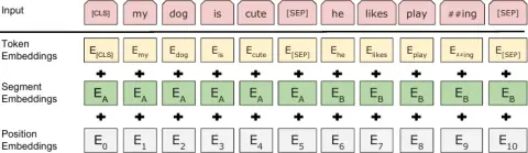
Given a sequence of words as inputs (limited to 512 tokens), BERT performs a first transformation of these words in order to obtain numerical input representations to pass to the model. In practice, these input representations are constructed by summing three different types of embedding: token, segment and positional embeddings. A visualization of this construction can be seen in Figure 8.

2.2.1. Token Embedding

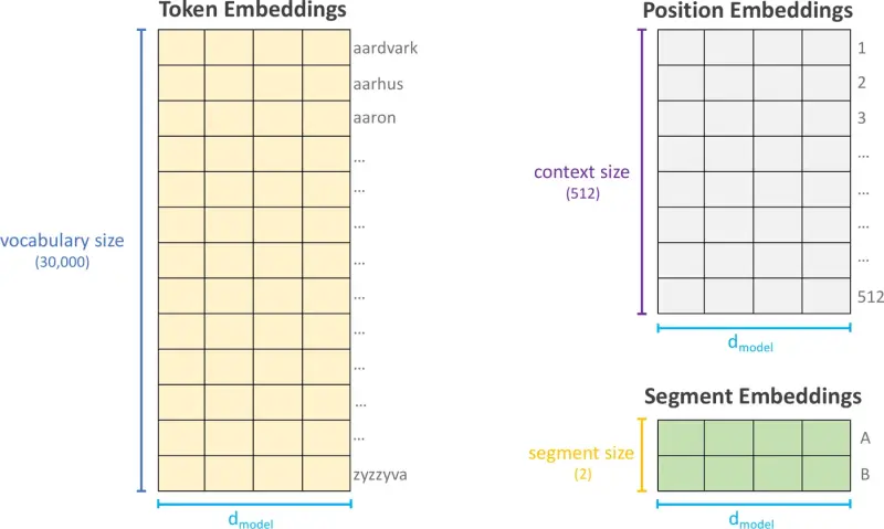
Given a word in the input sequence, BERT uses WordPiece embedding⁸ to tokenize it. Basically, WordPiece is a model that creates a fixed-size vocabulary of individual characters, subwords and words that best fits a given language corpus. To tokenize a word under this model, the tokenizer first checks if the whole word is in the vocabulary. If not, it tries to break it into the largest possible subwords contained in the vocabulary, and as a last resort will decompose the word into individual characters. Once the word has been processed into one or multiple WordPiece tokens, the vocabulary ids of these tokens are used to retrieve the corresponding embeddings in the learned token embedding matrix, shown in Figure 9.

The vocabulary used by BERT contains the \(\sim\)30,000 most common words and subwords found in the English language, in addition to all English characters and three special tokens:

• [CLS], which is used as a special classification token that appears at the beginning of every sequence. The final hidden state corresponding to this token is used as the aggregate sequence representation for classification tasks. It is ignored in non-classification tasks.
• [SEP], which is used as a delimiter when dealing with sentence pairs packed together into a single sequence. It also always ends the sequence.
• [MASK], which is used for the masked language modeling (MLM) training objective, discussed in the Masked Language Modeling section.

2.2.2. Segment Embedding

When dealing with sentence pairs, a learned segment embedding is added to every token indicating whether it belongs to sentence A or sentence B. Segment embeddings are similar to token embeddings with a simple vocabulary of size 2, as illustrated in Figure 9.

2.2.3. Positional Embedding

In order to inject some information about the relative or absolute position of the tokens in the input sequence, BERT uses positional embeddings, as in the original Transformer. These embeddings have the same dimension \(d_{\mathrm{model}}\) as the token and segment embeddings so that they can easily be summed up. They are computed using sine and cosine functions of different frequencies:

where \(pos\) is the position and \(i\) is the dimension. Hence, each dimension of the positional embedding corresponds to a sinusoid, and the wavelengths form a geometric progression from \(2\pi\) to \(10000 \cdot 2\pi\). Vaswani et al.³ hypothesized that this function allows the model to easily learn the relative positions, since for any fixed offset \(k\), \(\operatorname{PE}_{pos+k}\) can be represented as a linear function of \(\operatorname{PE}_{pos}\).

2.3. Parameters

As mentioned earlier, BERT comes in two versions. The base version has about 110M parameters in total, while the large one has 340M parameters in total. These parameters include:

• the token, positional and segment embedding matrices of the input embedding layer, respectively defined as

  \[\boldsymbol{W}^{TE} \in \mathbb{R}^{d_{\text{voc}} \times d_{\mathrm{model}}}, \boldsymbol{W}^{PE} \in \mathbb{R}^{d_{\text{context}} \times d_{\mathrm{model}}}, \boldsymbol{W}^{SE} \in \mathbb{R}^{2 \times d_{\mathrm{model}}}.\]

• the query, key and value weight matrices of each self-attention sublayer, respectively defined as

  \[\boldsymbol{W}^{Q} \in \mathbb{R}^{d_{\text{model}} \times d_k}, \boldsymbol{W}^{K} \in \mathbb{R}^{d_{\text{model}} \times d_k}, \boldsymbol{W}^{V} \in \mathbb{R}^{d_{\text{model}} \times d_v}.\]

• the \(h\) triplets of multi-head linear projections in each self-attention sublayer (where \(h\) refers to the number of attention heads), defined as

  \[\left(\boldsymbol{P}_{i}^{Q} \in \mathbb{R}^{d_{\text{model}} \times d_k}, \boldsymbol{P}_{i}^{K} \in \mathbb{R}^{d_{\text{model}} \times d_k}, \boldsymbol{P}_{i}^{V} \in \mathbb{R}^{d_{\text{model}} \times d_v}\right), \hspace{0.4cm} i=1,...,h.\]

• the multi-head output projection matrix in each self-attention sublayer, defined as

  \[\boldsymbol{W}^{O} \in \mathbb{R}^{d_{\text{model}} \times d_{\text{model}}}.\]

• the feed-forward network parameters in each feed-forward sublayer, defined as

  \[\left(\boldsymbol{W}_{1} \in \mathbb{R}^{d_{\text{model}} \times d_{\text{ff}}}, \boldsymbol{b}_{1} \in \mathbb{R}^{d_{\text{ff}}}\right), \left(\boldsymbol{W}_{2} \in \mathbb{R}^{d_{\text{ff}} \times d_{\text{model}}}, \boldsymbol{b}_{2} \in \mathbb{R}^{d_{\text{model}}}\right).\]

• the residual connection parameters in each layer, defined as

  \[\boldsymbol{W}^R \in \mathbb{R}^{d_{\text{model}}}.\]

In practice, we have

A visualization of all these parameters is given in Figure 9 and Figure 10. Additionally, a detailed breakdown of BERT parameters is given in the thesis appendix for the base and large versions.

(a) Parameters of a Self-Attention sublayer.

(b) Parameters of a FFN sublayer.

3. Pre-training Procedure

BERT is pre-trained simultaneously on two tasks: masked language modeling (MLM) and next sentence prediction (NSP). The training loss is simply the sum of the mean MLM likelihood and the mean NSP likelihood.

3.1. Masked Language Modeling

Unlike language modeling (LM), which aims at predicting the next word given the sequence of previous words, masked language modeling is the task of predicting a percentage of input tokens which are randomly masked.

The MLM training objective was chosen over the traditional LM objective because of the bidirectionality of BERT (i.e., BERT uses both left and right context in the sequence to predict the target word). For such models, standard conditional language modeling cannot be used as training objective, as the bidirectional conditioning would allow each word to indirectly “see itself”, and the model could trivially predict the target word in a multi-layered context. Hence, BERT is trained using masked language modeling, also referred as a Cloze task in the literature⁹. As shown in Figure 11, the prediction is given by the final hidden vectors corresponding to the masked tokens, that are fed into an output softmax over the vocabulary, as in a standard LM.

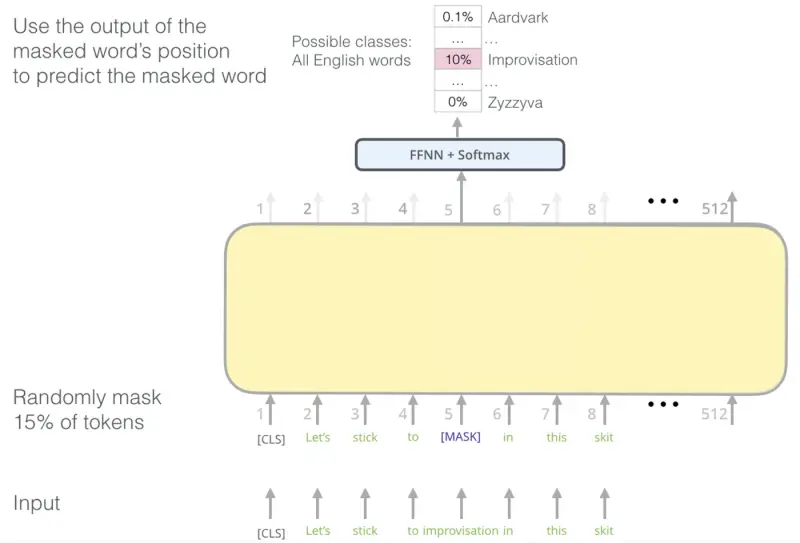
Formally, given an input sequence \(\boldsymbol{x}=[x_1,x_2,...,x_N]\) of \(N\) tokens, MLM first selects a random set of \(k\) positions (integers between 1 and \(N\)) to mask out \(\boldsymbol{m}=[m_1,...,m_k]\). The tokens in the selected positions are then replaced with a [MASK] token, resulting in the masked input sequence \(\boldsymbol{x}^{\mathrm{masked}}\). BERT eventually learns to predict the original identities of the \(k\) masked-out tokens by computing an output word distribution \(\hat{\boldsymbol{y}}^{(h)}\) \((h=1,...,k)\) for each one of them. More precisely, given the \(h\)-th masked word \(x_{m_h}\) from sequence \(\boldsymbol{x}\), the MLM loss function is the cross-entropy between the predicted probability distribution \(\hat{\boldsymbol{y}}^{(h)}\), and the true next word distribution \(\boldsymbol{y}^{(h)}\), which is simply the one-hot vector for \(x_{m_h}\). Therefore, we have

The overall loss of the sequence is simply the average loss for all the \(k\) masked-out tokens in \(\boldsymbol{x}^{\mathrm{masked}}\),

The masking procedure works as follows: BERT selects 15% of all WordPiece tokens in each training sequence at random. If the \(i\)-th token is chosen, it is replaced with:

1. the [MASK] token 80% of the time;
2. a random token 10% of the time;
3. the unchanged \(i\)-th token 10% of the time.

The selected words are not always replaced with the [MASK] token because it would then create a mismatch between pre-training and fine-tuning, since the masked token would never be seen before fine-tuning.

3.2. Next Sentence Prediction

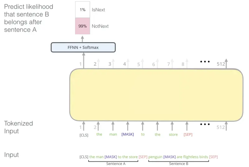
Next sentence prediction (NSP) is a binary classification task in which the model receives pairs of sentences as input and learns to predict if the second sentence in the pair is the subsequent sentence in the original corpus. This training objective helps understand the relationship between pairs of sentences, which is not directly captured by language modeling but still very important for many downstream tasks such as question-answering (QA) and natural language inference (NLI).

This prediction task can can be easily generated from any monolingual corpus. Specifically, when choosing the sentences A and B for each pre-training example, 50% of the time B is the actual next sentence that follows A (labeled as IsNext), and the other 50% of the time it is a random sentence from the corpus (labeled as NotNext). In this case, the final hidden vector corresponding to the [CLS] token is fed into an output softmax over the two possible predictions, as shown in Figure 12.

4. Downstream Tasks

There are two strategies for applying pre-trained language representations to downstream NLP tasks: fine-tuning and feature-based. On one hand, the fine-tuning approach introduces minimal task-specific parameters, and is trained on the downstream tasks by simply fine-tuning all pre-trained parameters. On the other hand, the feature-based approach uses task-specific architectures that include the pre-trained representations as input features for learning the task.

4.1. Fine-tuning Approach

The two pre-training objectives of BERT allow it to be used on any single sequence and sequence-pair tasks without substantial task-specific architecture modifications. For each task, one only needs to plug in the task-specific inputs and outputs into BERT and fine-tune all the parameters end-to-end for a few epochs. Figure 13 illustrates the fine-tuning of BERT on different common tasks.

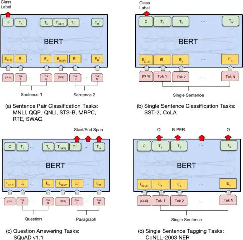
At the input, sentence A and sentence B from pre-training are similar to:

1. sentence pairs in paraphrasing;
2. hypothesis-premise pairs in entailment;
3. question-passage pairs in question-answering;
4. a degenerate text-\(\varnothing\) pair in text classification or sequence tagging.

At the output, the token representations are fed into an output layer for token-level tasks (e.g., sequence tagging or question-answering), and the [CLS] representation is fed into an output layer for text classification (e.g., entailment or sentiment analysis).

4.2. Feature-based Approach

In addition to the fine-tuning approach, where a simple output layer is added to the pre-trained model and all parameters are jointly fine-tuned on a downstream task, BERT can also be used with a feature-based approach, where word representations are extracted from the pre-trained model and serve as inputs to other task-specific architectures. This approach has certain advantages over the fine-tuning one. First, not all tasks can be easily represented by a Transformer encoder architecture, and therefore require a task-specific model architecture to be added. Second, there are major computational benefits to pre-compute an expensive representation of the training data once and then run many experiments with cheaper models on top of this representation.

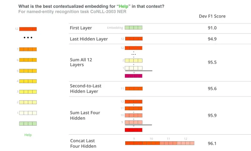
There are several ways of extracting contextual word embeddings from BERT representations, and which approach works best mainly depends on the task it is being evaluated on. For example, Devlin et al.¹ led a study for the task of named entity recognition (NER), where they applied a feature-based approach by extracting the activations from one or more layers without fine-tuning any parameters of BERT on the task, and then used these contextual embeddings as inputs to a randomly initialized two-layer 768-dimensional BiLSTM before the classification layer. The results showed that concatenating the last four hidden layers as the contextual word embeddings led to the best F1 scores for that specific task, as shown in Figure 14.

References