A brief intro to word embeddings

A word embedding is a dense, fixed-length, real-valued vector representation of a word. More formally, an embedding model is a parameterized function \(\mathcal{W} \rightarrow \mathbb{R}^n\) that maps every word \(w \in \mathcal{W}\) to a point in a high-dimensional vector space.

Word embeddings have become a core component of natural language processing (NLP) systems. Text is composed of units such as words and characters, but computers cannot interpret those symbols in a human sense. To process language with machine-learning models, we first need to turn it into numerical representations. Ideally, those representations should capture useful semantic and syntactic properties rather than merely assign an arbitrary number to every word.

The simplest approach is one-hot encoding. Given a vocabulary of \(N\) words, we assign an index \(i \in \{1, \ldots, N\}\) to each word. A word is then represented by an \(N\)-dimensional vector containing zeros everywhere except at its index, where the value is one.

One-hot vectors are easy to construct, but they have two major limitations. First, their dimensionality grows with the vocabulary: more dimensions mean more parameters, more training data, and more computation. Second, they encode no similarity between words. Any two distinct one-hot vectors are equally distant, whether they represent cat and dog or cat and database. A useful embedding space should instead place semantically related words near one another.

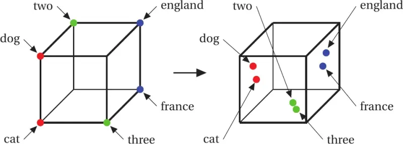
This goal is closely related to the distributional hypothesis, introduced by Zellig S. Harris: words that occur in similar contexts tend to have similar meanings.¹ John R. Firth later summarized the idea with the famous observation that a word is characterized by the company it keeps.²

Most embedding methods rely on this principle in one way or another. They can be organized into three broad families:

• Count-based models derive representations from corpus-wide co-occurrence statistics.
• Prediction-based models learn representations by predicting a word from its context, or the context from a word.
• Deep contextual models generate a different representation for a token depending on the sentence in which it appears.

1. Count-based models

Count-based models start with a co-occurrence matrix. This matrix is built by scanning a large collection of documents and recording how frequently words occur together.

Two common variants are:

• A word-document matrix \(\mathbf{X} \in \mathbb{N}^{N \times D}\), where \(N\) is the vocabulary size, \(D\) is the number of documents, and \(\mathbf{X}_{ij}\) records how often word \(i\) appears in document \(j\).
• A window-based matrix \(\mathbf{X}' \in \mathbb{N}^{N \times N}\), where \(\mathbf{X}'_{ij}\) records how often word \(i\) occurs within a fixed-size context window around word \(j\).

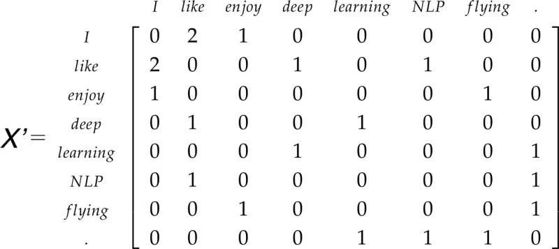
Because these matrices are large and sparse, their dimensionality is usually reduced. One classical approach is Singular Value Decomposition (SVD), which factorizes the matrix as

The rows of a truncated \(\mathbf{U}\) matrix can then serve as compact word embeddings. Well-known count-based approaches include Latent Semantic Analysis (LSA),³ Hyperspace Analogue to Language (HAL),⁴ Correlated Occurrence Analogue to Lexical Semantics (COALS),⁵ and Hellinger PCA.⁶

These models use global corpus statistics effectively and often capture word similarity well. However, they generally perform less well on relationships such as analogies, suggesting that their vector spaces do not encode every kind of linguistic structure equally well.

2. Prediction-based models

Prediction-based approaches do not construct embeddings directly from a count matrix. Instead, they learn representations as parameters of a model trained to predict words from their context.

2.1. Neural network language model

The neural network language model proposed by Bengio and colleagues jointly learns word vectors and a statistical language model.⁷ It uses a feed-forward neural network with a linear projection layer and a non-linear hidden layer.

Given a sequence of words \(w_1, \ldots, w_n\) from a vocabulary \(V\), the objective is to estimate the probability of the next word from the preceding words:

The model can be understood as the composition of two mappings, \(C\) and \(g\):

• \(C\) is the embedding lookup table. In practice, it is a \(\lvert V\rvert \times m\) matrix of learned parameters mapping each word index to an \(m\)-dimensional vector.
• \(g\) receives the context vectors and returns a probability distribution over the vocabulary for the next word, typically through a softmax layer.

Training maximizes the average log-likelihood of the corpus:

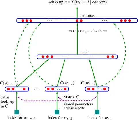
The principal drawback is the final softmax layer. Computing a probability for every possible output word has a cost proportional to \(\lvert V\rvert\), which may contain hundreds of thousands or even millions of entries. Training such a model can therefore be computationally expensive.

2.2. Continuous bag-of-words

The continuous bag-of-words model (CBOW), one of the two original Word2Vec architectures, predicts a target word from the words surrounding it.⁸ Unlike a standard language model, it can use context on both sides of the target because its purpose is to learn useful word representations rather than generate text from left to right.

For a context window of size \(n\), its objective can be written as

CBOW removes the non-linear hidden layer of the earlier feed-forward language model, reducing its computational cost. Let \(\mathbf{W} \in \mathbb{R}^{\lvert V\rvert \times d}\) denote the weights between the input and projection layers. Each row of \(\mathbf{W}\) is the \(d\)-dimensional representation of one vocabulary word.

For a one-hot input vector \(\mathbf{x}\) whose non-zero entry is at position \(k\),

The multiplication simply selects the corresponding row of the embedding matrix. With multiple context words, CBOW averages their representations:

A second matrix \(\mathbf{W}' \in \mathbb{R}^{d \times \lvert V\rvert}\) maps the hidden representation to an output score for every vocabulary word:

The softmax operation turns these scores into a probability distribution:

Once training is complete, \(\mathbf{W}\), \(\mathbf{W}'\), or an average of the two can be used as the final word embedding matrix.

2.3. Skip-gram

The skip-gram model reverses the CBOW prediction task: instead of predicting the center word from its context, it predicts the surrounding words from the center word.⁸

Its objective sums the log probabilities of the words within a context window of radius \(c\):

The transition from the input to the projection layer works as in the single-word CBOW case: the one-hot input selects one row of \(\mathbf{W}\). The difference lies in the output, where the model predicts multiple context-word distributions rather than a single center word.

(a) Continuous bag-of-words model.

(b) Skip-gram model.

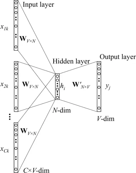
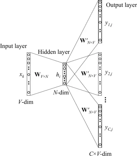
CBOW and skip-gram form Word2Vec.⁹ Their success came not only from these simple architectures but also from efficient approximations to the full softmax, most notably negative sampling and hierarchical softmax.⁸

Negative sampling updates the model using a small set of sampled words rather than summing over the entire vocabulary. Hierarchical softmax organizes the output vocabulary as the leaves of a binary tree, reducing probability computation to a path through that tree. Both techniques make large-scale embedding training considerably faster.¹⁰

Skip-gram also forms the basis of FastText.¹¹ Instead of learning only one vector per word, FastText represents a word through character n-grams and combines their representations. For example, with \(n=3\), artificial contains sequences such as art, rti, and tif. This subword structure enables the model to construct representations for rare or previously unseen words, something standard Word2Vec cannot do directly.

3. Deep contextual models

Count-based models and Word2Vec assign one fixed vector to each word. That representation captures the word’s most common usages across the training corpus, but it cannot resolve polysemy: the same spelling may have different meanings in different contexts. The word bank, for example, should not have exactly the same representation in river bank and investment bank.

Deep contextual models address this limitation by assigning each token a representation that depends on the entire input sentence. Early contextual approaches included Context2Vec,¹² CoVe,¹³ ELMo,¹⁴ and ULMFiT,¹⁵ many of which used bidirectional recurrent networks to encode context.

The Transformer architecture¹⁶ subsequently enabled a new generation of pretrained contextual language models, including BERT,¹⁷ XLNet,¹⁸ and ERNIE.¹⁹ Unlike static embedding methods, these models can produce different vectors for the same word according to its surrounding words. That ability to represent meaning in context is one of the reasons pretrained language models have proved effective across such a wide range of NLP tasks.

References