An illustrated intro to Transformers

Download the original presentation (PDF)

1. From text to vectors

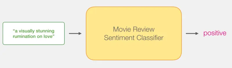
A familiar natural language processing task is sentiment classification: the model receives a piece of text as input and and outputs a predefined sentiment class (positive, negative, or neutral).

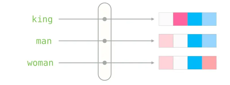
Neural networks cannot operate directly on words. Text must first be mapped to vectors. A word embedding provides such a mapping, ideally in a space where useful semantic and syntactic relationships are reflected geometrically.

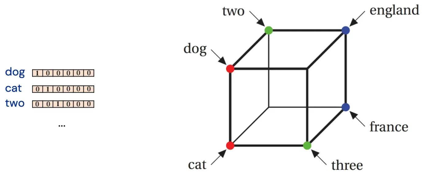
The simplest representation is one-hot encoding. Given a vocabulary of \(N\) words, one-hot encoding consists in assigning an integer index \(i \in \{1,\ldots,N\}\) to each word such that the word is represented as an \(N\)-dimensional sparse vector mostly composed of zeros, except for a single entry at the position corresponding to the word’s index in the vocabulary that takes the value 1. In addition to suffering from an obvious feature size downside, this approach does not take similarities between words into account.

Distributional methods learn more useful spaces from the contexts in which words appear. As J. R. Firth summarized the idea: “You shall know a word by the company it keeps.” Well-known and largely used word embedding methods such as Word2Vec (Mikolov et al., 2013), GloVe (Pennington et al., 2014) and FastText (Bojanowski et al., 2016), all have a major weakness though: they create a fixed embedding for each word. Therefore, whatever the meaning of the word, it will always be mapped to the same vector.

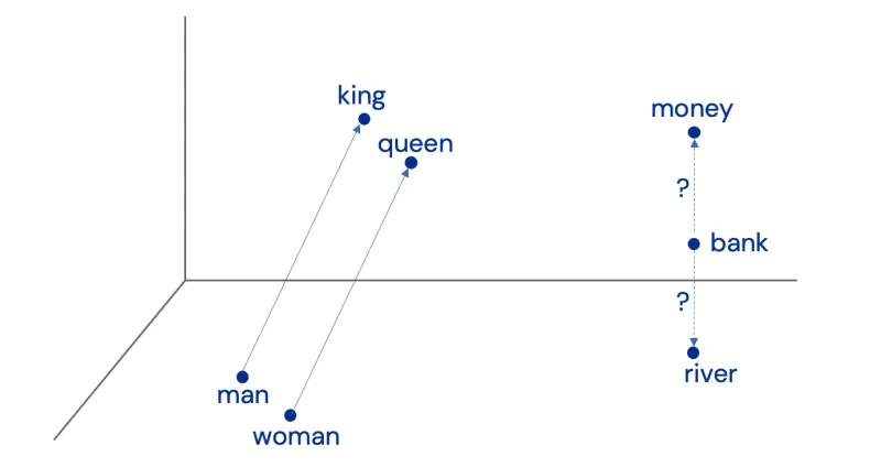
The limitation of one fixed vector per word motivates contextual representations. The Transformer constructs them with self-attention.

2. Self-attention

As the model processes a certain word from the input sequence, self-attention allows the model to attend to all the other words from the sequence for clues to a good contextual representation of that word. In the example below, the model can associate it with animal rather than street.

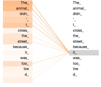
Self-attention is produced in six steps:

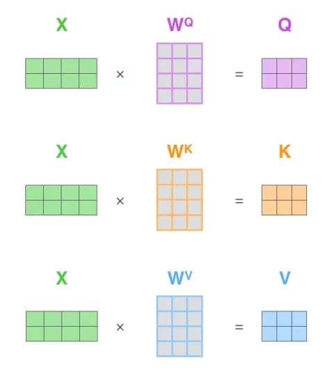
• Step 1: Create a query, key, and value vector for each input word. These vectors are obtained by multiplying an initial word embedding vector (learned during training) by three distinct weight matrices \(\boldsymbol{W}^{Q}\), \(\boldsymbol{W}^{K}\), and \(\boldsymbol{W}^{V}\) (also learned during training).

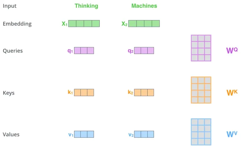
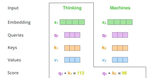
• Step 2: Given a word of the input sequence, score its query vector with the key vectors of all other words. Scores are calculated by computing the dot product of the query-key vectors.

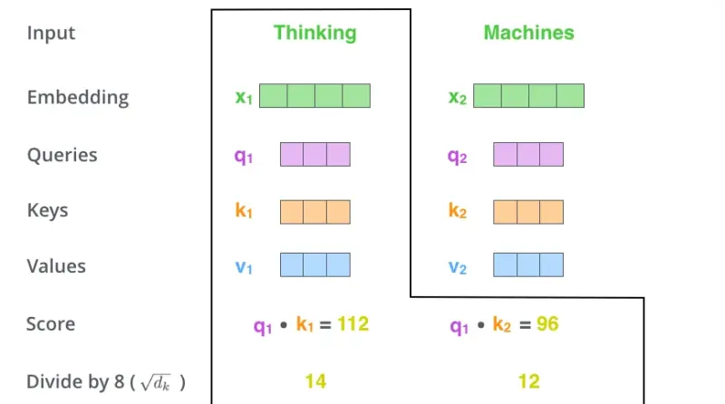
• Step 3: Divide the scores by the square root of the key vector dimension. This division leads to more stable gradients.

• Step 4: Pass all the scores through a softmax operation. Softmax normalizes the scores so they are all positive and add up to 1.

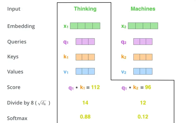
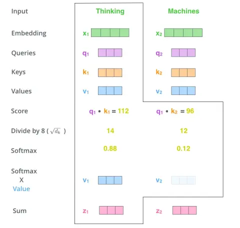
• Step 5: Multiply each value vector by its softmax score. The intuition here is to keep intact the value vectors of the word(s) the model decides to focus on, and drown out those of irrelevant words.

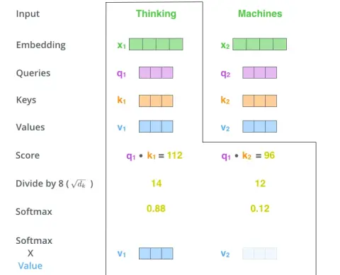
• Step 6: Sum up all weighted value vectors. This produces the output vector of the self-attention calculation for a given word in the input sequence.

In practice, the tokens are processed together: packing the input embeddings into a matrix \(\boldsymbol{X}\) and multiplying it by the respective weight matrices \(\boldsymbol{W}^{Q}\), \(\boldsymbol{W}^{K}\), and \(\boldsymbol{W}^{V}\).

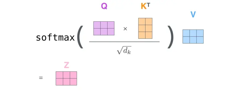
Steps 2 to 6 can be condensed in one formula.

3. Multi-head attention

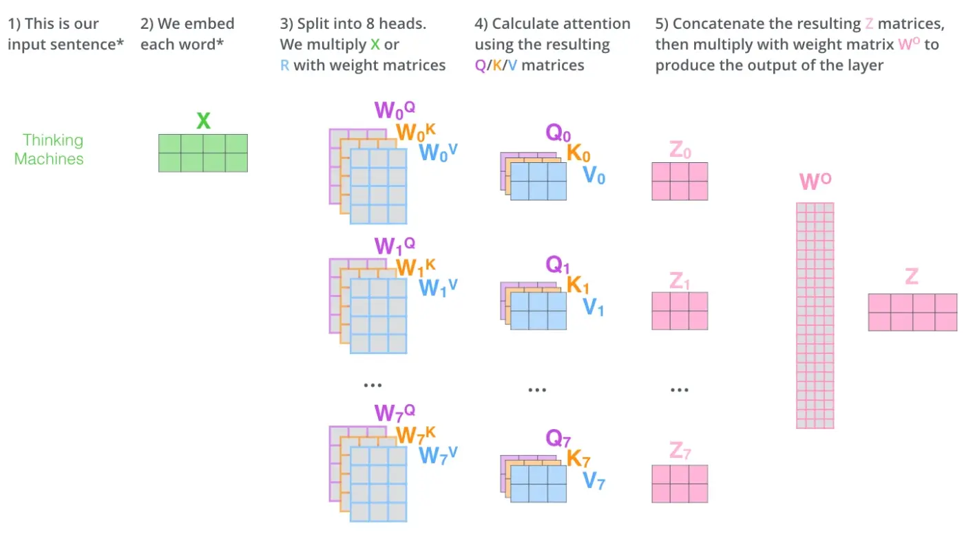
In the Transformer architecture, the self-attention computation is performed several times on each input word using different sets of Query/Key/Value weight matrices. Each of these sets is called an attention head and the whole mechanism is called multi-head attention. Separate \(\boldsymbol{W}^{Q}\), \(\boldsymbol{W}^{K}\), and \(\boldsymbol{W}^{V}\) matrices are maintained for each attention head.

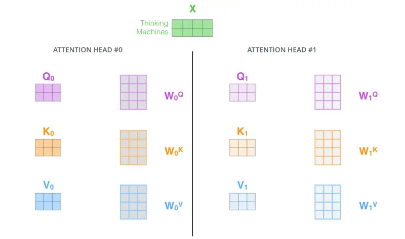
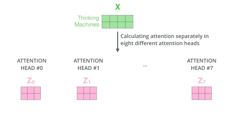
The Transformer uses 8 attention heads. The different self-attention calculations result in 8 different output matrices \(\boldsymbol{Z}_i\).

The final output from the self-attention layer is obtained by concatenating the different \(\boldsymbol{Z}_i\) matrices and multiplying them by a weight matrix \(\boldsymbol{W}^{O}\).

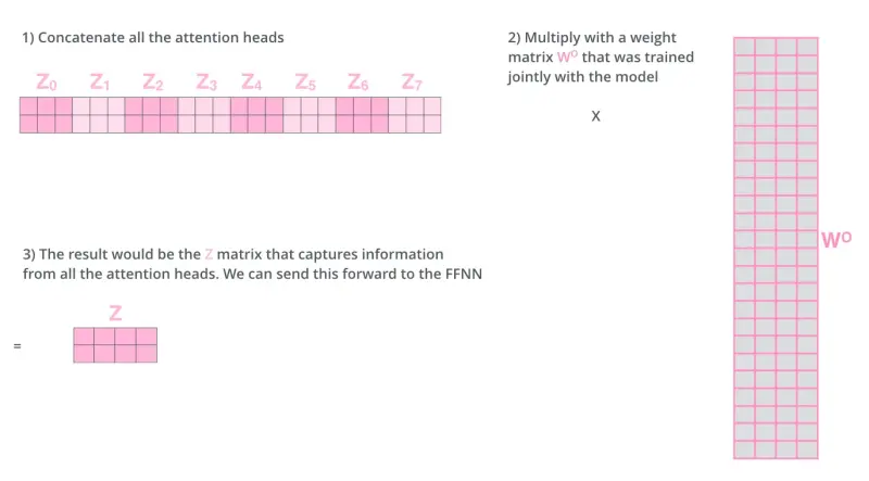
The complete multi-head attention computation is illustrated below.

4. Transformer

The Transformer⁵ architecture is composed of an encoder and a decoder.

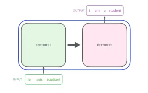
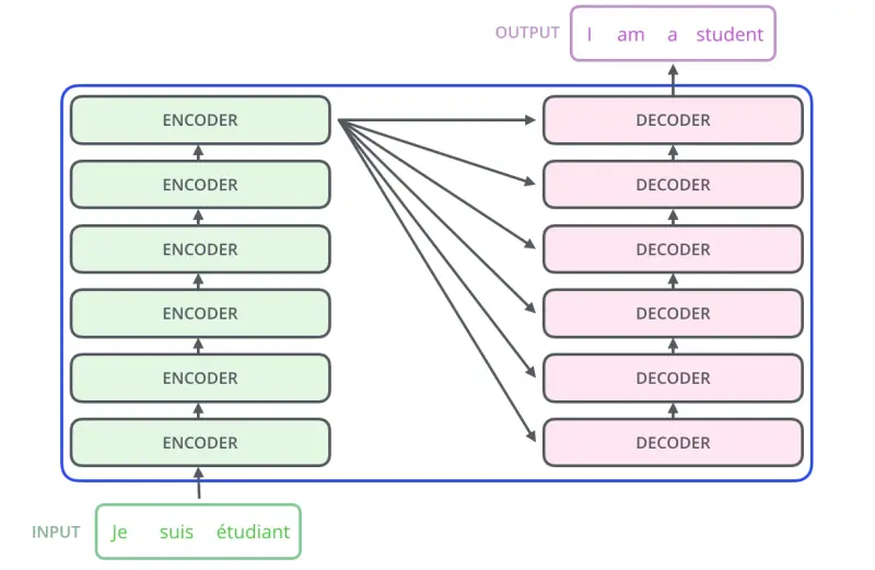
Both the encoder and decoder are stacks of several encoding and decoding layers respectively, all identical in structure but not sharing the same weights.

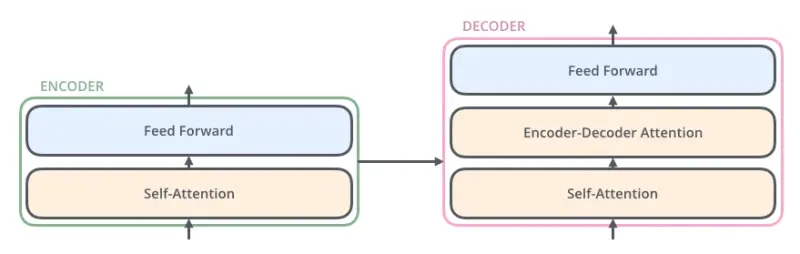
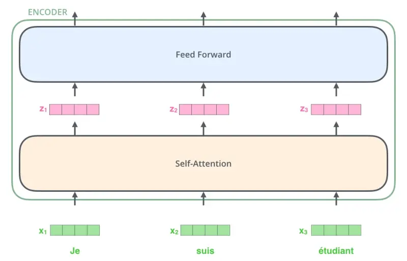
Each encoder layer contains two types of sub-layers: (1) a self-attention layer that helps look at other words in the sequence when encoding a given word, and (2) a shallow feed-forward layer that is independently applied to each word vector, allowing the various paths to be executed in parallel.

Each decoder layer contains an extra sub-layer in-between: (3) an encoder-decoder attention layer, which helps focus on relevant parts of the initial input sequence.

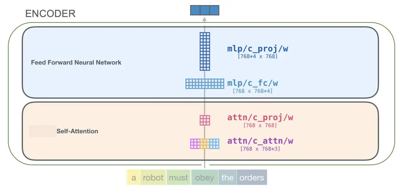
Every block in a Transformer has its own weights:

1. the weight matrix used to create the queries, keys, and values (attn/c_attn/w);
2. the weight matrix that projects the results of the attention heads into the output vector of the self-attention sub-layer (attn/c_proj/w);
3. the weight matrix corresponding to the first layer of the Feed Forward Neural Network (mlp/c_fc/w);
4. the weight matrix corresponding to the second layer of the Feed Forward Neural Network (mlp/c_proj/w).

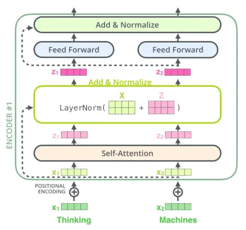
Each sub-layer in an encoder/decoder layer has a residual connection around it, followed by a layer-normalization step.

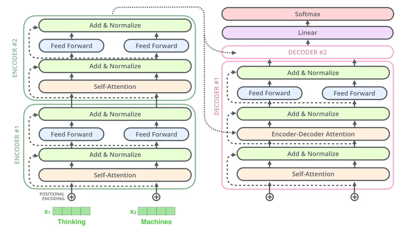
After each sub-layer, the output matrix \(\boldsymbol{Z}\) is added to the input matrix \(\boldsymbol{X}\) and the result is normalized.

Before being given to the encoder, each word must be converted to an input vector.

The Transformer uses a data-driven tokenization method that creates a fixed-size vocabulary of individual characters, sub-words and words that best fits a given language corpus.

For example, the WordPiece tokenization model first checks if the full word is in the vocabulary. If not, it tries to break it down into the largest possible sub-words from the vocabulary. As a last resort, it decomposes the word into individual characters.

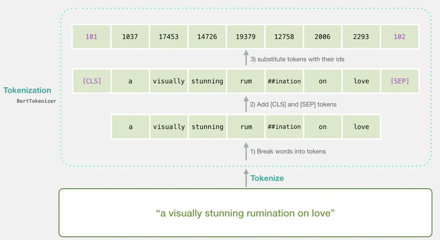
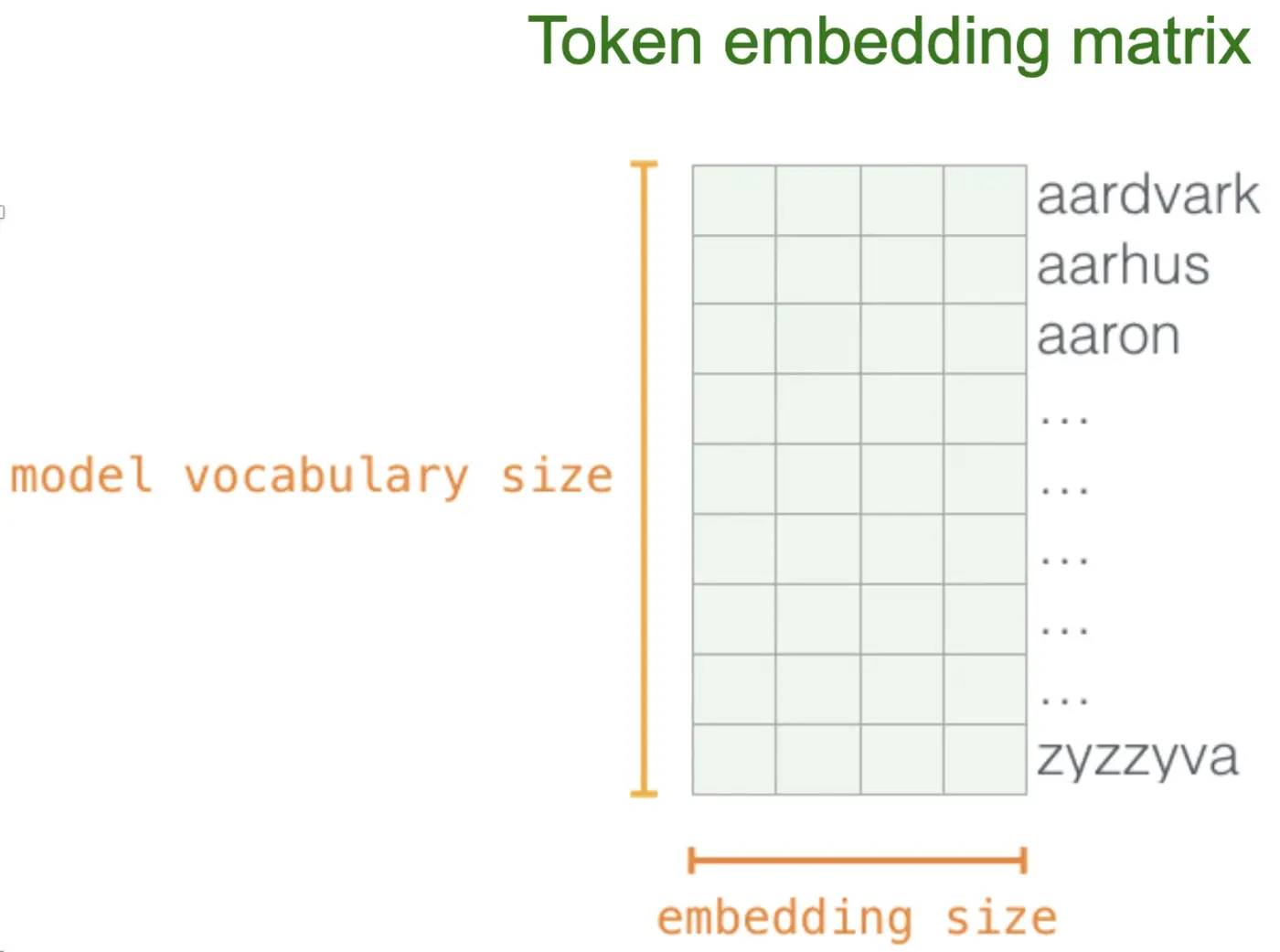
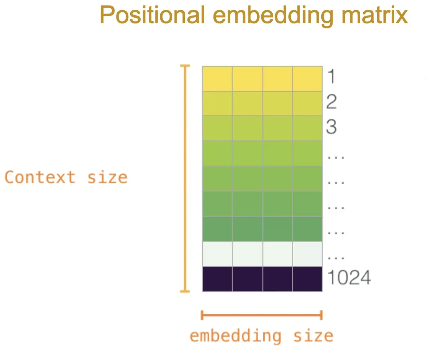
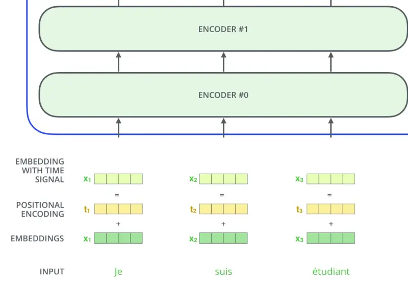
To give the model a sense of order of the input words, positional encoding vectors are added to the token vectors. This results in the final input embedding that goes to the encoder.

The output of the last encoder layer is transformed into a set of attention vectors \(\boldsymbol{K}\) and \(\boldsymbol{V}\), resulting from the multiplication of the FFN output matrix \(\boldsymbol{R}\) with the weight matrices \(\boldsymbol{W}^{K}\) and \(\boldsymbol{W}^{V}\).

Matrices \(\boldsymbol{K}\) and \(\boldsymbol{V}\) are used by each decoder layer in its encoder-decoder attention sub-layer, which works just like the self-attention sub-layer except it creates the query matrix \(\boldsymbol{Q}\) from the sub-layer below it and takes the key and value matrices from the output of the encoder stack. This sub-layer helps the decoder focus on appropriate positions from the initial input sequence.

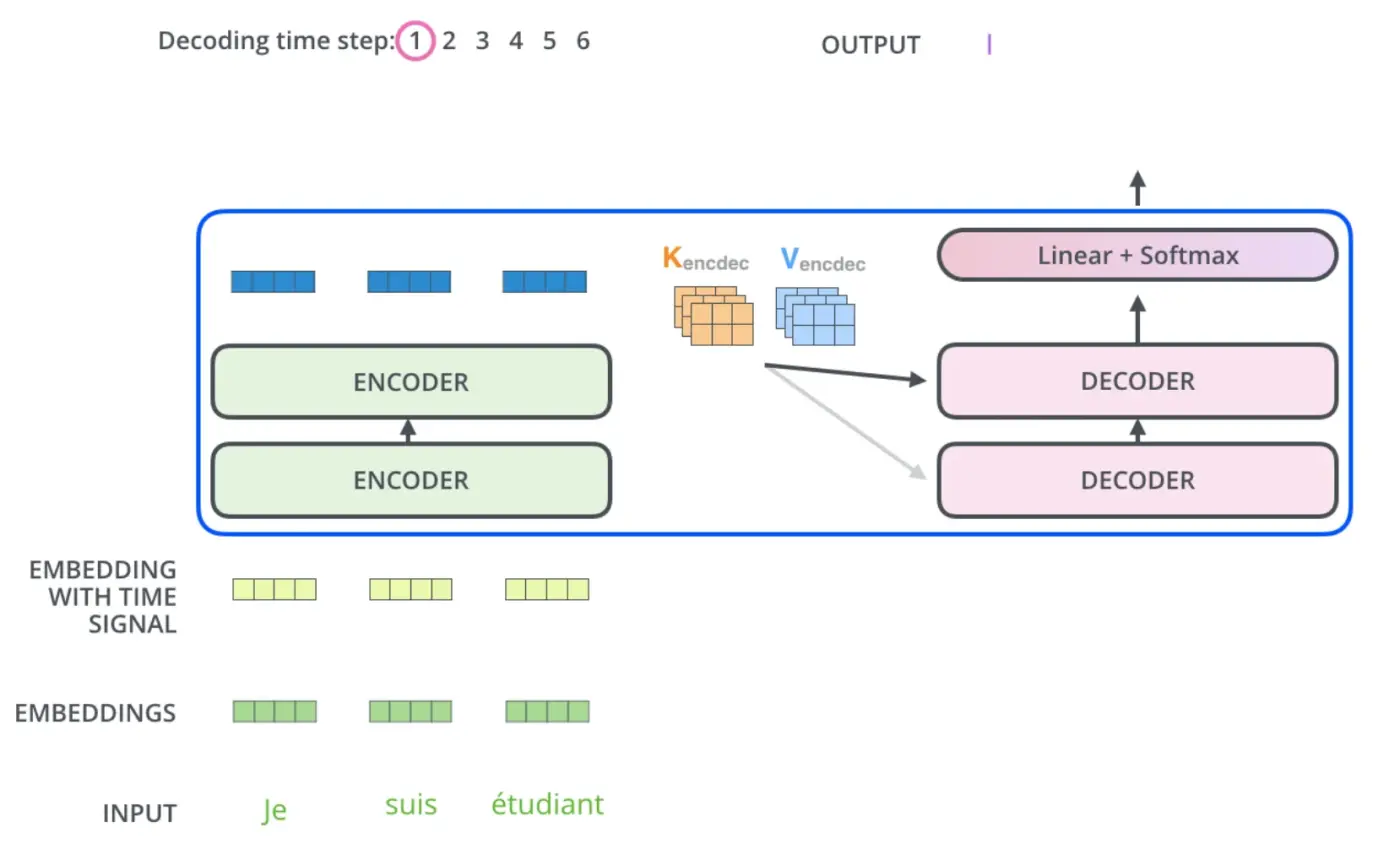
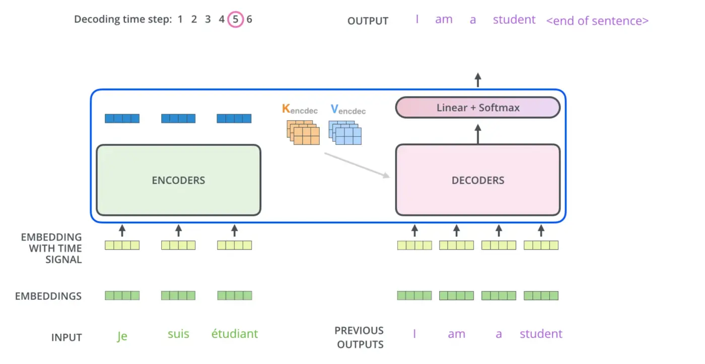
The decoder output of each step is fed back to the decoder as input for the next time step. Note that the self-attention sub-layer in the decoder is only allowed to attend to earlier positions from the output sequence. This is done by masking future positions (setting them to \(-\infty\)) before the softmax step in the self-attention calculation.

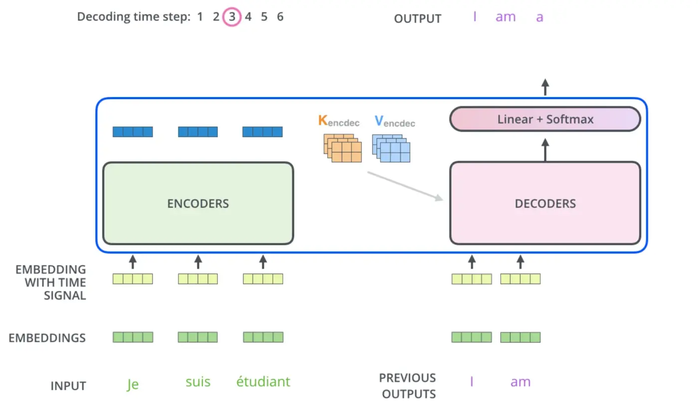
The decoding process continues until a special symbol is reached indicating that the decoder has completed its output.

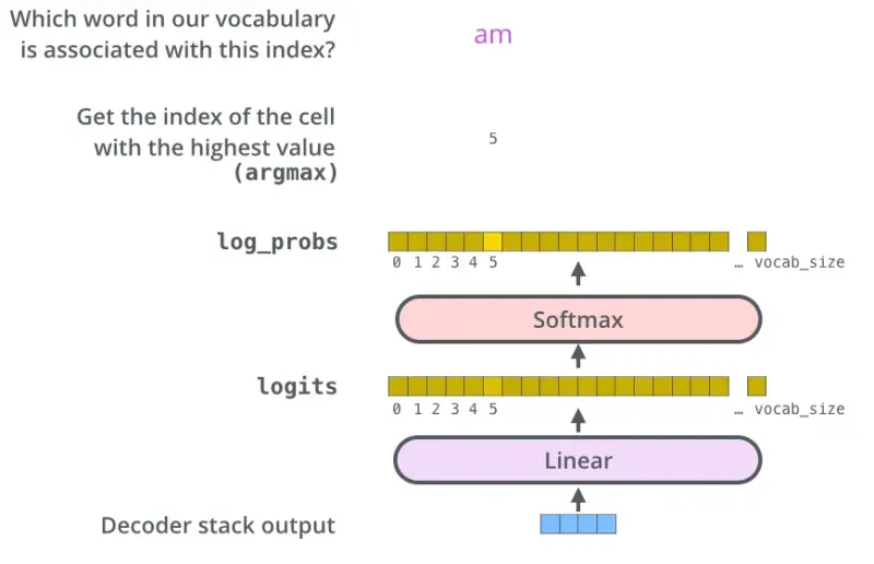
The linear sub-layer is a simple fully connected neural network that projects the vector produced by the stack of decoders into a much larger vector of the size of the vocabulary (logits vector). Intuitively, each cell of the logits vector corresponds to the score given to the corresponding word. The softmax then turns those scores into probabilities. The cell with the highest probability is chosen and the word associated to it is the output for that time step.

5. BERT

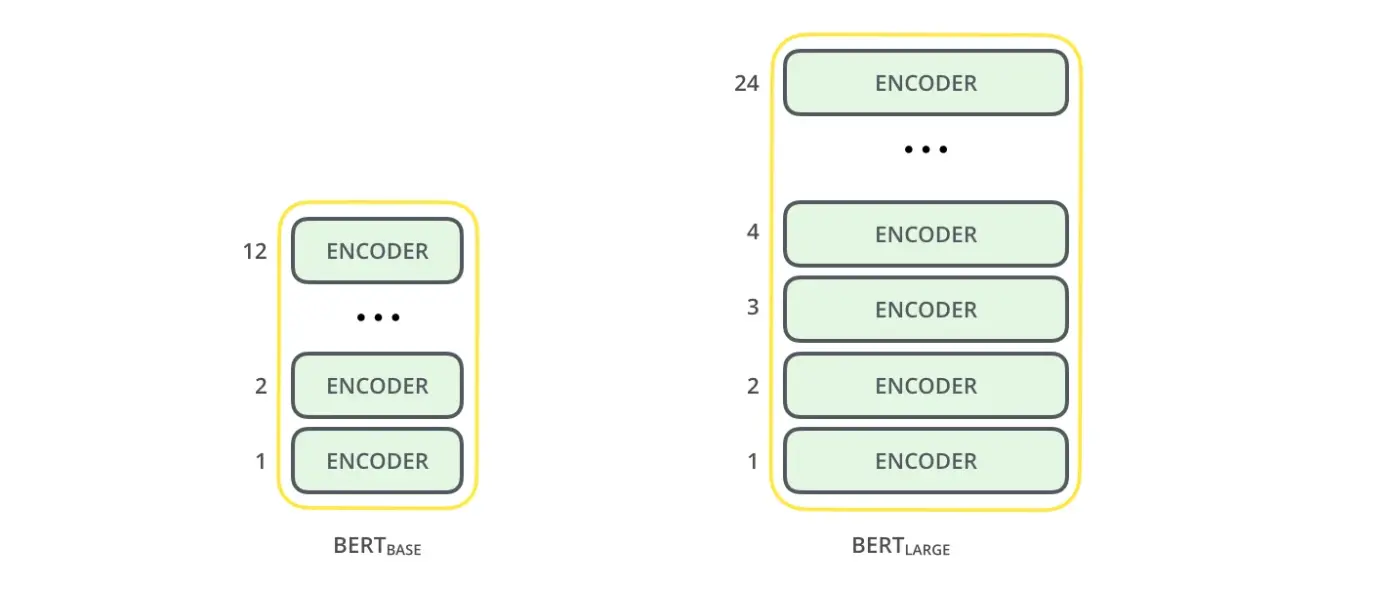
BERT⁷ is a pre-trained Transformer encoder with 12 layers for its BASE model and 24 for its LARGE version (compared to 6 for the Transformer). BERT also has a larger hidden size (768 and 1024 for \(BERT_{BASE}\) and \(BERT_{LARGE}\) respectively, compared to 512 for the original Transformer), larger feed-forward sub-layers (3072 and 4096 units, compared to 2048), and more attention heads (12 and 16, compared to 8).

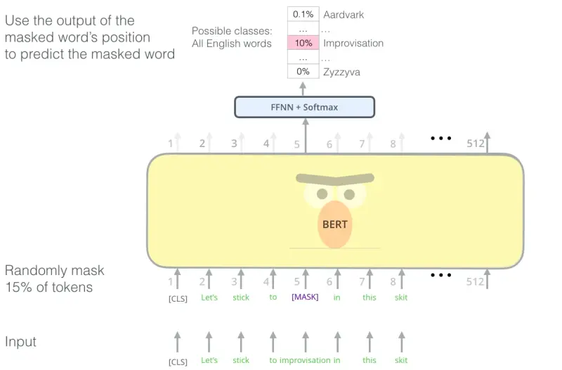
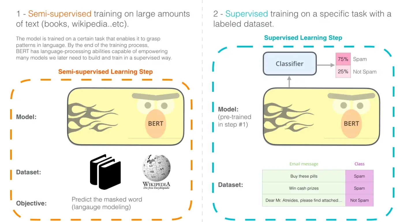
The first task BERT is pre-trained on is masked language modeling. Before feeding word sequences into BERT, 15% of the words in each sequence are replaced with a [MASK] token. The model then attempts to predict the original value of the masked words based on the context provided by the other, non-masked, words in the sequence.

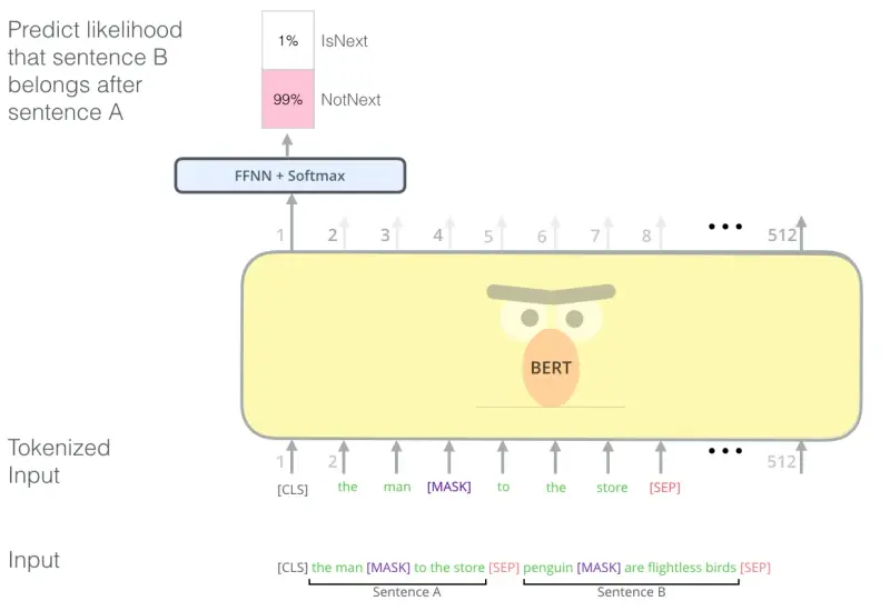
The second task BERT is pre-trained on is a two-sentence classification task. In BERT’s training process, the model receives pairs of sentences as input and learns to predict whether the second sentence in the pair follows the first one.

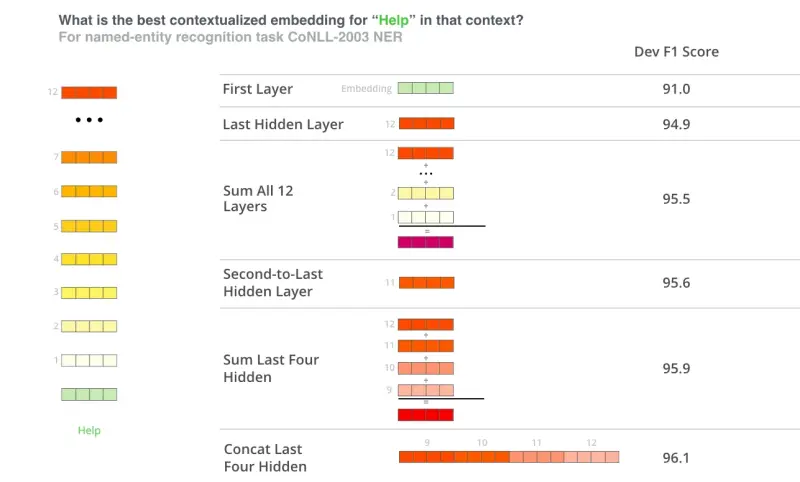
Once pre-trained, BERT’s output can be used as contextualized word embeddings. One can choose among multiple options to get the embedding of a word: summing up, averaging, or concatenating all or some layers’ outputs.

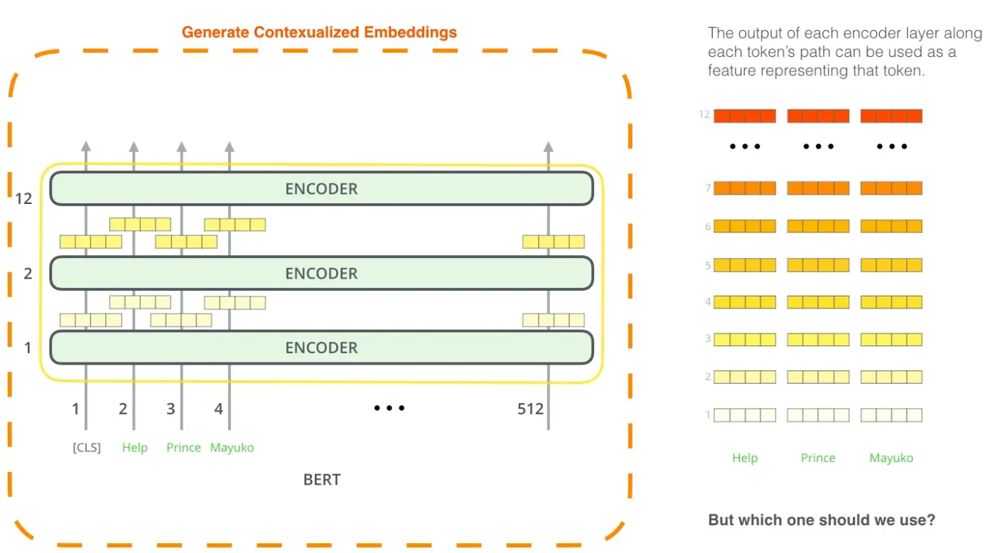
Which vector works best as a contextualized embedding depends on the task. The example below reports results for Named Entity Recognition (NER) on the CoNLL-2003 dataset.

BERT obtained new state-of-the-art results on 11 natural language processing tasks.

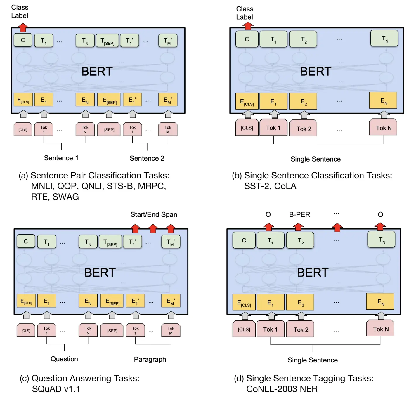
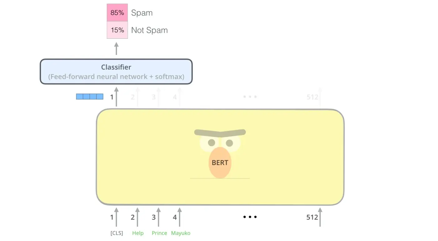
The first input token is supplied with a special [CLS] token (standing for “classification”) and is used for classification tasks where only the output vector of this special token is sent to the classifier.

BERT uses a two-step fine-tuning approach:

References and credits