Transformer & Friends
This (in-progress) post aims to stay up-to-date with the popular Transformer-based models.
Table of contents
- Transformer
- BERT [to come]
Transformer
The Transformer (Vaswani et al., 2017) is undoubtedly one of the most impactful works in recent years. It took the NLP world by surprise by achieving state-of-the-art results in almost every language task, and it is now doing the same for audio and vision. The model secret recipe is carried in its architecture and so-called “self-attention” mechanism.
Self-attention
Attention (Bahdanau et al., 2014) is a mechanism to be learned by a neural network that relates elements in a source sequence to a target sequence by selectively concentrating on a relevant set of the information at hand. The amount of attention put on each element is given by the learned weights and the final output is usually a weighted average.
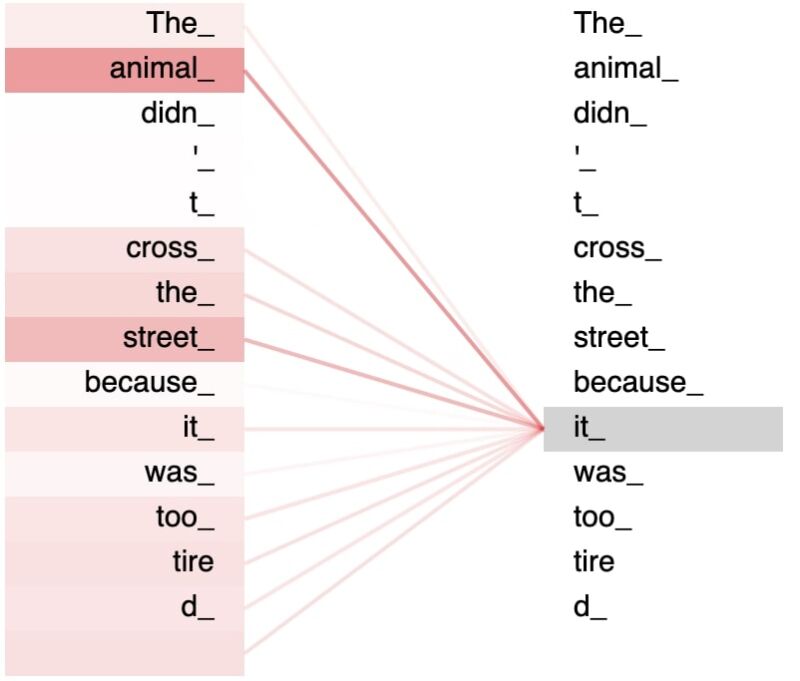
Self-attention is a type of attention mechanism that relates different elements of a single sequence (source and target are the same).
The Transformer model relies on the scaled dot-product attention. Given a set of query, key, and value vectors (one of each for every term in the input sequence), the output vector of a given term is a weighted sum of all the value vectors in the sequence, where the weight assigned to each value is determined by the dot-product of the query vector with the corresponding key vector.
For each term \(t_i\) of an input sequence \(\{t_1, \cdots, t_n\}\), the self-attention mechanism performs the following steps:
-
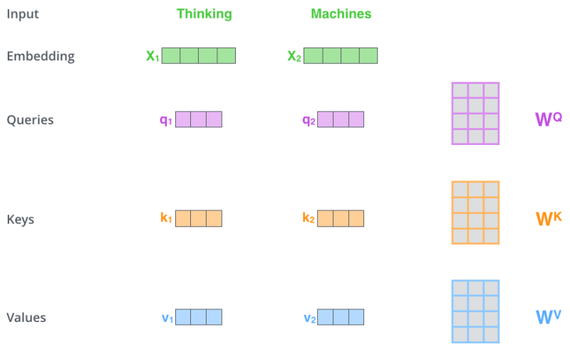
Query, key, value. Compute the query, key, and value vectors by multiplying the initial term embedding \(\boldsymbol{x}_i \in \mathbb{R}^{d_{\text{model}}}\) with the query weight matrix \(\boldsymbol{W}^{Q} \in \mathbb{R}^{d_{\text{model}} \times d_{k}}\), the key weight matrix \(\boldsymbol{W}^{K} \in \mathbb{R}^{d_{\text{model}} \times d_{k}}\), and the value weight matrix \(\boldsymbol{W}^{V} \in \mathbb{R}^{d_{\text{model}} \times d_{v}}\), respectively: \(\begin{equation} \begin{aligned} \boldsymbol{q}_i &= \boldsymbol{x}_i \boldsymbol{W}^Q, \\ \boldsymbol{k}_i &= \boldsymbol{x}_i \boldsymbol{W}^K, \\ \boldsymbol{v}_i &= \boldsymbol{x}_i \boldsymbol{W}^V, \end{aligned} \end{equation}\)
-
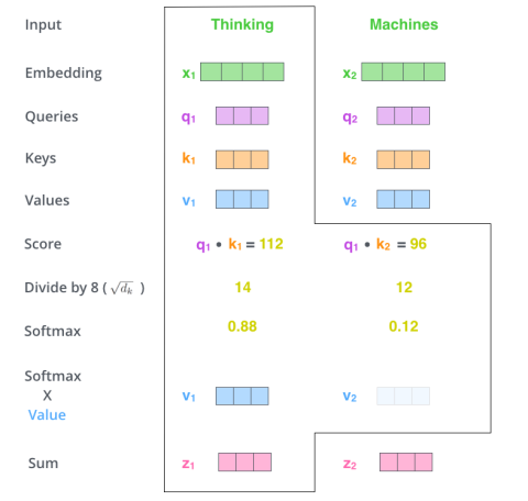
Alignment scores. Score term \(t_i\) against all the other terms in the sequence by taking the dot-product of its query vector with all the key vectors of the sequence: \(\begin{equation} s_{ij} = \frac{\boldsymbol{q}_i \boldsymbol{k}_j}{\sqrt{d_k}}, \hspace{1cm} \forall j=1,...,n. \end{equation}\) NB: Dividing the scores by the square root of the key vector dimension aims at providing the dot-products to grow large in magnitude when \(d_k\) is large, which has the effect to push the softmax result into regions where it has extremely small gradients.
-
Weights. Normalize the alignment scores by applying a softmax operation: \(\begin{equation} \alpha_{ij} = \frac{e^{s_{ij}}}{\sum_{j=1}^{n} e^{s_{ij}}}, \hspace{1cm} \forall j=1,...,n. \end{equation}\)
-
Context vector. Sum up the weighted value vectors as the final context vector: \(\begin{equation} \boldsymbol{z}_i = \sum_{j=1}^{n} \alpha_{ij} \boldsymbol{v}_{j}. \end{equation}\)
In practice, the self-attention mechanism is computed on a set of queries simultaneously, packed together into a matrix \(\boldsymbol{Q} \in \mathbb{R}^{n \times d_k}\). The keys and values are also packed together into respective matrices \(\boldsymbol{K} \in \mathbb{R}^{n \times d_k}\) and \(\boldsymbol{V} \in \mathbb{R}^{n \times d_v}\). The output matrix is then computed as follows: \(\begin{equation} \text{Attention}(\boldsymbol{Q},\boldsymbol{K},\boldsymbol{V}) = \text{softmax}\left(\frac{\boldsymbol{Q}\boldsymbol{K}^\top}{\sqrt{d_k}}\right)\boldsymbol{V}. \end{equation}\)
Multi-Head Self-Attention
Rather than computing the self-attention once, the Transformer uses the so-called “multi-head” attention mechanism, where self-attention is performed in parallel on \(h\) different linear projections of the query, key and value matrices. This yields \(h\) different output matrices \(\boldsymbol{Z}_i \in \mathbb{R}^{n \times d_{\mathrm{model}}}\) called “attention heads”, which are then concatenated and projected into a final representation subspace: \(\begin{equation} \begin{aligned} \operatorname{MultiHead}(\boldsymbol{Q}, \boldsymbol{K}, \boldsymbol{V}) &=\text{Concat}\left(\boldsymbol{Z}_{1}, \ldots, \boldsymbol{Z}_{\mathrm{h}}\right) \boldsymbol{W}^{O} \\ \text{with } \boldsymbol{Z}_{\mathrm{i}} &=\text{Attention}\left(\boldsymbol{Q} \boldsymbol{P}_{i}^{Q}, \boldsymbol{K} \boldsymbol{P}_{i}^{K}, \boldsymbol{V} \boldsymbol{P}_{i}^{V}\right), \end{aligned} \end{equation}\) where \(\boldsymbol{P}_{i}^{Q} \in \mathbb{R}^{d_{\text {model }} \times d_{k}}\), \(\boldsymbol{P}_{i}^{K} \in \mathbb{R}^{d_{\text {model }} \times d_{k}}\), \(\boldsymbol{P}_{i}^{V} \in \mathbb{R}^{d_{\text {model }} \times d_{v}}\), and \(\boldsymbol{W}^{O} \in \mathbb{R}^{hd_{v} \times d_{\text{model}}}\) are parameter matrices to be learned. According to the paper, “multi-head attention allows to jointly attend to information from different representation subspaces at different positions”.

Encoder-Decoder Architecture
[…]